Simulating Molecules(LiH) Using VQE
The path you have taken isn’t for the faint hearted
Qiskit Summer School Final Project: Designing your implementation of a variational quantum eigensolver (VQE) algorithm that simulates the ground state energy of the Lithium Hydride (LiH) molecule.

INTRODUCTION
Fundamentally, light was believed to be a wave. However, Albert Einstein found that light consisted of photons called quanta, which have energy determined by its frequency. Photons of visible light can be absorbed by an electron, thereby causing the electron to move from a low energy orbital to a high energy orbital.
Determining these properties is difficult for a classical computer since the electrons may be highly entangled. To model this accurately, we require more computational power, and this is where quantum computers come into play. Compared to classical computers, they are more efficient at handling entanglement.
LiH is a 12 body molecule containing 4 protons, 4 electrons, and 4 neutrons. This creates a 12 body model, which becomes intractable when simulating it both with a classical and quantum computer. So, this model reduces the First Quantized Molecular Hamiltonian to one two body interaction between two electrons in the hybridized p orbital and four one body interactions with their respective nuclei.

One of the essential properties is the ground state energy of a molecule. Finding the ground state energy of these molecules becomes harder as the size of the molecule increases, which is why until now, the largest simulated molecule is Beryllium Hydride. Molecular simulations’ problems grow exponentially as the size of molecules increase. Some of the applications of these problems are in drug discoveries.
Richard Feynman said, “Nature isn’t classical, dammit, and if you want to make a simulation of nature, you’d better make it quantum mechanical, and by golly, it’s a wonderful problem because it doesn’t look so easy.”
PROCESS
The variational principle explains how the energy of any trial wave function is greater than or equal to the system’s exact ground state energy.
It is important to find the minimum eigenvalue of a matrix; in Chemistry, the minimum eigenvalue of a Hermitian matrix is the ground state energy.

1. We map the molecular Hamiltonians into qubit Hamiltonians. We find the fermionic operators and map the fermionic Hamiltonians to qubit Hamiltonians. For this transformation we use
1. Jordan Wigner transformation leads to N-local Hamiltonians
2. Bravyi-Kotoev transformation leads to log(N) local Hamiltonians
3. Partity transformation
We then copy the electron orbitals interactions to qubits.
2. We create an ansatz.
The expectation value of any wave function will be at least the minimum eigenvalue associated with the wave function.
The ground state of the Hamiltonian system is the smallest eigenvalue associated with the Hermitian matrix.
3. Parameter optimization
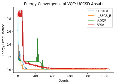
One problem that arises is noise, meaning the energy calculations may not be true. We try and overcome this by gradient descent, which also has its problems. We use Simultaneous Perturbation Stochastic Approximation (SPSA) as the ideal optimizer. It works by perturbing all the parameters in random. Under noise, Sequential Least Squares Programming (SLSQP) and Constrained Optimization BY Linear Approximation (COBYLA) are preferred.
IMPLEMENTATION
Notebook is here
Defining your molecule:
In this challenge, we will focus on LiH using the sto3g basis with the PySCF driver, which can be described in Qiskit as follows: ‘inter_dist’ is the interatomic distance.
inter_dist = 1.6
driver = PySCFDriver(atom=‘Li .0 .0 .0; H .0 .0’ + str(inter_dist), unit=UnitsType.ANGSTROM, charge=0, spin=0, basis=‘sto3g’)
We also set up the molecular orbitals to be considered and can reduce the problem size when we map to the qubit Hamiltonian. Hence, the amount of time required for the simulations is reasonable for a laptop computer.
# please be aware that the idx here with respective to original idx
freeze_list = [0]
remove_list = [-3, -2] # negative number denotes the reverse order
Now, you can start choosing the components that make up your VQE algorithm!
1. Optimizers
The most commonly used optimizers are COBYLA, L_BFGS_B, SLSQP, and SPSA.
2. Qubit mapping
There are several different mappings for your qubit Hamiltonian, parity, bravyi_kitaev, jordan_wigner, which in some cases can allow you to reduce the problem size further.
3. Initial state
There are different initial states that you can choose to start your simulation. Typically people choose from the zero state init_state = Zero(qubitOp.num_qubits) and the UCCSD initial state HartreeFock(qubitOp.num_qubits, num_spin_orbitals, num_particles, map_type, qubit_reduction)
4. Parameterized circuit
There are different choices you can make in the form of variational forms of your parameterized circuit.
UCCSD_var_form = UCCSD(num_qubits, depth=depth, num_orbitals=num_spin_orbitals, num_particles=num_particles)
RY_var_form = RY(num_qubits, depth=depth)
RYRZ_var_form = RYRZ(num_qubits, depth=depth)
swaprz_var_form = SwapRZ(num_qubits, depth=depth)
5. Simulation backend
There are different simulation backends that you can use to perform your simulation.
backend = BasicAer.get_backend('statevector_simulator')
backend = Aer.get_backend('qasm_simulator')
Compare the convergence of different choices for building your VQE algorithm
Among the above choices, which combination do you think would outperform others and give you the lowest estimation of LiH ground state energy with the quickest convergence? Compare the results of different combinations against each other and the classically computed exact solution at a fixed interatomic distance, for example, inter_dist=1.6.
To access the intermediate data during the optimization, you would need to utilize the callback option in the VQE function:
counts = []
values = []
params = []
deviation = []
def store_intermediate_result(eval_count, parameters, mean, std):
counts.append(eval_count)
values.append(mean)
params.append(parameters)
deviation.append(std)
algo = VQE(qubitOp, var_form, optimizer, callback=store_intermediate_result)
algo_result = algo.run(quantum_instance)
Compute the ground state energy of LiH at various interatomic distances
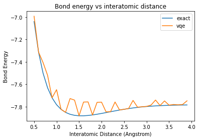
By changing the parameter inter_dist, you can use your VQE algorithm to calculate the ground state energy of LiH at various interatomic distances, and potentially produce a plot as you see here. Note that the VQE results are very close to the exact results, and so the exact energy curve is hidden by the VQE curve.
NOTE: I am not using the noisy model
distances = np.arange(0.5, 4.0, 0.1)
exact_energies = []
vqe_energies = []
for dist in distances:
qubitOp, num_spin_orbitals, num_particles, qubit_reduction, shift = compute_LiH_qubitOp(map_type=‘parity’, inter_dist=dist)
# Classically solve for the exact solution and use that as your reference value
ref = exact_solver(qubitOp) + shift
# Specify your initial state
init\_state = HartreeFock(num\_spin\_orbitals, num\_particles, "parity", qubit\_reduction)

# Select a state preparation ansatz
# Equivalently, choose a parameterization for our trial wave function.
var\_form = UCCSD(num\_orbitals=num\_spin\_orbitals,
                 num\_particles=num\_particles,
                 initial\_state=init\_state,
                 qubit\_mapping="parity")

# Choose where to run/simulate our circuit
quantum\_instance = Aer.get\_backend('statevector\_simulator')

# Choose the classical optimizer
optimizer = SPSA()

# Run your VQE instance
vqe = VQE(qubitOp, var\_form, optimizer, callback=store\_intermediate\_result)

# Now compare the results of different compositions of your VQE algorithm!

ret = vqe.run(quantum\_instance)
vqe\_result = np.real(ret\['eigenvalue'\]) + shift
print("Interatomic Distance:", np.round(1.4, 2), "VQE Result:", vqe\_result, "Exact Energy:", ref)
exact\_energies.append(ref)
vqe\_energies.append(vqe\_result)
plt.plot(np.arange(0.5, 4.0, 0.1), exact_energies, label=“exact”)
plt.plot(np.arange(0.5, 4.0, 0.1), vqe_energies, label=“vqe”)
plt.xlabel(‘Interatomic Distance (Angstrom)’)
plt.ylabel(‘Bond Energy’)
plt.legend()
plt.title(‘Bond energy vs interatomic distance’)
plt.show()
# Dictionary of optimizers:
opt_dict = {‘SPSA’ , ‘SLSQP’ , ‘COBYLA’ , ‘L_BFGS_B’}
for opt in opt_dict:
print(‘Testing’, str(opt) , ‘optimizer’)
qubitOp, num_spin_orbitals, num_particles, qubit_reduction, shift = compute_LiH_qubitOp(map_type , 1.5)
# Classically solve for the exact solution and use that as your reference value
ref = exact_solver(qubitOp) + shift
# Specify your initial state
init\_state = HartreeFock(num\_spin\_orbitals,num\_particles, qubit\_mapping='parity')

# Select a state preparation ansatz
# Equivalently, choose a parameterization for our trial wave function.
var\_form = UCCSD(num\_orbitals=num\_spin\_orbitals, num\_particles=num\_particles, qubit\_mapping='parity')

# Choose where to run/simulate our circuit
quantum\_instance = Aer.get\_backend('statevector\_simulator')

# Choose the classical optimizer
if opt == 'SPSA':
    optimizer = SPSA(max\_trials = 500)
elif opt == 'SLSQP':
    optimizer = SLSQP(maxiter = 1000)
elif opt == 'L\_BFGS\_B':
    optimizer = L\_BFGS\_B(maxfun = 1000 ,  maxiter = 1000)
elif opt == 'COBYLA':
    optimizer = COBYLA(maxiter = 1000)

counts =\[\]
values =\[\]
params =\[\]
deviation =\[\]

# Run your VQE instance
vqe = VQE(qubitOp, var\_form, optimizer , callback = store\_intermediate\_result)
vqe\_results = vqe.run(quantum\_instance)

#Printing error in final value:
ground\_state\_energy = vqe\_results\['eigenvalue'\] + shift
energy\_error\_ground = np.abs(np.real(ref) - ground\_state\_energy)
print('Error:', str(energy\_error\_ground))
# Calculating energy error
vqe\_energies = np.real(values) + shift
energy\_error = np.abs(np.real(ref) - vqe\_energies)
plt.plot(counts , energy\_error , label=str(opt))
plt.legend()
plt.xlabel(‘Counts’)
plt.ylabel(‘Energy Error/ Hartree’)
plt.title(‘Energy Convergence of VQE: UCCSD Ansatz’)
# Trying all combinations to get the most efficiency
maps_types = [‘parity’] # For ‘bravyi_kitaev’, ‘jordan_wigner’ we need another noise model eg ibmq_16_melbourne or ibmq_qasm_simulator
init_states = [“HartreeFock(num_spin_orbitals, num_particles, map_type, qubit_reduction)”,
“Zero(qubitOp.num_qubits)”]
var_forms = [“UCCSD(num_orbitals=num_spin_orbitals, num_particles=num_particles, active_occupied=[0], active_unoccupied=[0, 1], initial_state=init_state, qubit_mapping=map_type, two_qubit_reduction=qubit_reduction)”,
“RY(qubitOp.num_qubits, depth=depth)”,
“RYRZ(qubitOp.num_qubits, depth=depth)”,
“SwapRZ(qubitOp.num_qubits, depth=depth)”]
backends = [
“Aer.get_backend(‘qasm_simulator’)”]
optimizers = [“COBYLA(maxiter=opt_max_eval)”,
“L_BFGS_B(maxiter=opt_max_eval)”,
“SLSQP(maxiter=opt_max_eval)”,
“SPSA()”]
depth = 1
opt_max_eval = 200
for map_type in maps_types:
for i_state in init_states:
for v_form in var_forms:
for be in backends:
for opt in optimizers:
print(“map_type: “, map_type)
print(“i_state: “, i_state)
print(“v_form: “, v_form)
print(“be: “, be)
print(“opt: “, opt)
                qubitOp, num\_spin\_orbitals, num\_particles, qubit\_reduction = compute\_LiH\_qubitOp(map\_type, inter\_dist)
                # Classically solve for the exact solution and use that as your reference value
                ref = exact\_solver(qubitOp)

                # Specify your initial state
                init\_state = eval(i\_state)

                # Select a state preparation ansatz
                # Equivalently, choose a parameterization for our trial wave function.
                var\_form = eval(v\_form)

                # Choose where to run/simulate our circuit
                quantum\_instance = QuantumInstance(backend=eval(be),
                                                    noise\_model=noise\_model,
                                                    measurement\_error\_mitigation\_cls=CompleteMeasFitter,
                                                    seed\_simulator=167, seed\_transpiler=167,)

                # Choose the classical optimizer
                optimizer = eval(opt)

                # Run your VQE instance
                counts = \[\]
                values = \[\]
                params = \[\]
                deviation = \[\]
                algo = VQE(qubitOp, var\_form, optimizer, callback=store\_intermediate\_result)
                results = algo.run(quantum\_instance)
                print('VQE Results: {:.12f}'.format(results.eigenvalue.real))
                print('The total ground state energy is: {:.12f}'.format(results.eigenvalue.real))
                print("Parameters: {}".format(results.optimal\_point))

                #plt.plot(counts, label="count")
                plt.plot(values, label="Zero")
                plt.xlabel('Eval count')
                plt.ylabel('energy minimisation for various optimizers ')
                plt.legend()
                plt.show()

                #print(counts)
                #print(values)
                #print(params)
                #print(deviation)
                # Now compare the results of different compositions of your VQE algorithm!

                ## 8
                print("---")
Hopefully, you have gained a firm understanding of how VQE works and can now implement one on your own. Leave some claps and follow me for more content. I worked with Victor