Q1c. an Analysis of the Variational Quantum Classifier Using Data
Our previous blog is at: “Explaining Variational Quantum Classifiers”
By now you should know how a variational quantum classifier works. The code for the previous series is at Github repo
Introduction
In binary classification, let’s say labelling if someone is likely to have a heart attack or not, we would build a function that takes in the information about the patient and gives results aligned to the reality. E.g,

This probabilistic classification is well suited for quantum computing and we would like to build a quantum state that, when measured and post processed, returns

P(hear attack = YES)
By optimizing the circuits, you then find parameters that will give the closest probability to the reality based on training data.
Problem statement
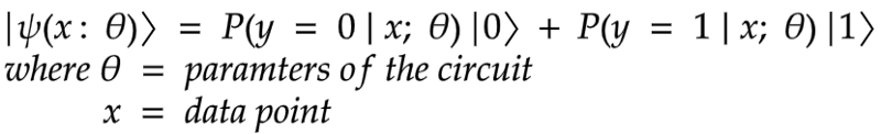
Given a dataset about patients’ information, can we predict if the patient is likely to have a heart attack or not? This is a binary classification problem, with a real input vector {x} and a binary output {y} in {0, 1}. We want to build a quantum circuit whose output is the quantum state:
Implementation
- We initialize our circuit in the zero state (all qubits in state zero)
self.sv = Statevector.from_label('0' * self.no_qubit)
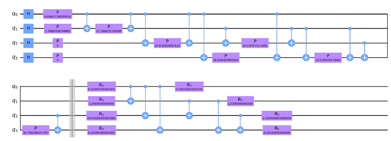
2. We use a feature map such as, ZZFeaturemap, ZFeaturemap or PauliFeaturemap and choose the number of qubits based on the input dimension of the data and how many repetitions (i.e. the circuit depth) we want. We use 1, 3, 5.
3. We choose the variational form as RealAmplitudes and specify the number of qubits as well as how many repetitions we want. We use 1, 2, 4 to have models with an increasing number of trainable parameters.
4. We then combine our feature map to the variational circuit. ZZfeaturemap and RealAmplitudes both with a depth of 1
def prepare_circuit(self):
"""
Prepares the circuit. Combines an encoding circuit, feature map, to a variational circuit, RealAmplitudes
:return:
"""
self.circuit = self.feature_map.combine(self.var_form)
5. We create a function that associates the parameters of the feature map with the data and the parameters of the variational circuit with the parameters passed. This is to ensure in Qiskit that the right variables in the circuit are associated with the right quantities.
def get_data_dict(self, params, x):
"""
Assign the params to the variational circuit and the data to the featuremap
:param params: Parameter for training the variational circuit
:param x: The data
:return parameters:
"""
parameters = {}
for i, p in enumerate(self.feature_map.ordered_parameters):
parameters[p] = x[i]
for i, p in enumerate(self.var_form.ordered_parameters):
parameters[p] = params[i]
return parameters
6. We create another function that checks the parity of the bit string passed. If the parity is even, it returns a ‘yes’ label and if the parity is odd it returns a ‘no’ label. We chose this since we have 2 classes and parity checks either returns true or false for a given bitstring. There are also other methods e.g for 3 classes you might convert the bistring to a number and pass is through an activation function. Or perhaps interpret the expectation values of a circuit as probabilities. The important thing to note is that there are multiple ways to assign labels from the output of a quantum circuit and you need to justify why or how you do this. In our case, the parity idea was originally motivated in this very nice paper (https://arxiv.org/abs/1804.11326) and the details are contained therein.
7. Now we create a function that returns the probability distribution over the model classes. After measuring the quantum circuit multiple times (i.e. with multiple shots), we aggregate the probabilities associated with ‘yes’ and ‘no’ respectively, to get probabilities for each label.
def return_probabilities(self, counts):
"""
Calculates the probabilities of the class label after assigning the label from the bit string measured
as output
:type counts: dict
:param counts: The counts from the measurement of the quantum circuit
:return result: The probability of each class
"""
shots = sum(counts.values())
result = {self.class_labels[0]: 0, self.class_labels[1]: 0}
for key, item in counts.items():
label = self.assign_label(key)
result[label] += counts[key] / shots
return result
8. Finally, we create a function that classifies our data. It takes in data and parameters. For every data point in the dataset we assign the parameters to the feature map and the parameters to the variational circuit. We then evolve our system and store the quantum circuit. We store the circuits so as to run them at once at the end. We measure each circuit and return the probabilities based on the bit string and class labels.
def classify(self, x_list, params):
"""
Assigns the x and params to the quantum circuit the runs a measurement to return the probabilities
of each class
:type params: List
:type x_list: List
:param x_list: The x data
:param params: Parameters for optimizing the variational circuit
:return probs: The probabilities
"""
qc_list = []
for x in x_list:
circ_ = self.circuit.assign_parameters(self.get_data_dict(params, x))
qc = self.sv.evolve(circ_)
qc_list += [qc]
probs = []
for qc in qc_list:
counts = qc.to_counts()
prob = self.return_probabilities(counts)
probs += [prob]
return probs
Results
Data classification was performed by using the implemented version of VQC in IBM’s framework and executed on the provider simulator
qiskit==0.23.1qiskit-aer==0.7.1qiskit-aqua==0.8.1qiskit-ibmq-provider==0.11.1qiskit-ignis==0.5.1qiskit-terra==0.16.1
Every combination of the experiments were executed with 1024 shots, using the implemented version of the optimizers. We conducted tests with different feature maps and depths, the RealAmplitudes variational form with differing depths and different optimizers in Qiskit. In each case, we compared the loss values after 50 training iterations on the training data. Our best model configs were
ZFeatureMap(4, reps=2) SPSA(max_trials=50) vdepth 5 : Cost: 0.13492279429495616ZFeatureMap(4, reps=2) SPSA(max_trials=50) vdepth 3 : Cost: 0.13842958846394343ZFeatureMap(4, reps=2) COBYLA(maxiter=50) vdepth 3 : Cost: 0.14097642258192988ZFeatureMap(4, reps=2) SPSA(max_trials=50) vdepth 1 : Cost: 0.14262128997684975ZFeatureMap(4, reps=1) COBYLA(maxiter=50) vdepth 1 : Cost: 0.1430145495411656ZZFeatureMap(4, reps=1) SPSA(max_trials=50) vdepth 5 : Cost: 0.14359757088670677ZFeatureMap(4, reps=2) COBYLA(maxiter=50) vdepth 5 : Cost: 0.1460568741051525ZFeatureMap(4, reps=1) SPSA(max_trials=50) vdepth 3 : Cost: 0.14830080135566964ZFeatureMap(4, reps=1) SPSA(max_trials=50) vdepth 5 : Cost: 0.14946706294763648ZFeatureMap(4, reps=1) COBYLA(maxiter=50) vdepth 3 : Cost: 0.15447151389989414
From the results, the ZFeatureMap with a depth of 2, RealAmplitudes variational form with a depth of 5 and the SPSA optimizer achieved the lowest cost. These results seem to indicate that the feature map which resulted in a lower cost function generally was the ZFeatureMap. But does this mean that the ZFeaturemap typically performs better in general?
Questions
1. Does increasing the variational form depth increase convergence?
- Interestingly, increasing the depth of the variational form does not seem to increase convergence of any of these models substantially. Note that increasing the variational form’s depth implies introducing more trainable parameters into the model. One would naively think that more parameters in the model would allow us to model things better and capture more intricate relationships that exist in the data, but perhaps these models are simply too small to exploit any of these advantages through higher parameterization.
2. Does increasing featuremap depth increase convergence?
- When increasing feature map depth on
ZZFeatureMap ADAM (maxiter=50)andPauliFeatureMap ADAM(maxiter=50), this does increase the convergence of model training. The other model configs don’t change significantly (in some, increasing the feature map depth actually reduces convergences almost linearly - why this happens could make for an interesting research project!).
3. How do the models generalize on different datasets?
- As a final experiment, we bench marked these results on the iris and wine datasets. Two popular datasets used in classical machine learning and of the same dimension of the heart attack data, hence we can also use 4 qubits to model it. This time, the best model configs were:
Iris dataset
PauliFeatureMap(4, reps=4) SPSA(max_trials=50) vdepth 3 : Cost: 0.18055905629600544ZZFeatureMap(4, reps=2) SPSA(max_trials=50) vdepth 5 : Cost: 0.18949957468013437ZFeatureMap(4, reps=2) SPSA(max_trials=50) vdepth 5 : Cost: 0.18975231416858743ZZFeatureMap(4, reps=1) SPSA(max_trials=50) vdepth 3 : Cost: 0.1916829328746686ZZFeatureMap(4, reps=4) SPSA(max_trials=50) vdepth 3 : Cost: 0.19264230430490895ZZFeatureMap(4, reps=2) SPSA(max_trials=50) vdepth 3 : Cost: 0.19356269726482855ZFeatureMap(4, reps=4) COBYLA(maxiter=50) vdepth 1 : Cost: 0.19415440209151674ZZFeatureMap(4, reps=4) SPSA(max_trials=50) vdepth 5 : Cost: 0.19598553766368446ZFeatureMap(4, reps=2) COBYLA(maxiter=50) vdepth 1 : Cost: 0.19703058320810934ZFeatureMap(4, reps=4) SPSA(max_trials=50) vdepth 3 : Cost: 0.19970277845347006
Wine dataset
PauliFeatureMap(4, reps=1) SPSA(max_trials=50) vdepth 5 : Cost: 0.1958180042610037PauliFeatureMap(4, reps=1) SPSA(max_trials=50) vdepth 3 : Cost: 0.1962278498243972PauliFeatureMap(4, reps=2) SPSA(max_trials=50) vdepth 3 : Cost: 0.20178754496022344ZZFeatureMap(4, reps=2) SPSA(max_trials=50) vdepth 1 : Cost: 0.20615090555639448PauliFeatureMap(4, reps=2) SPSA(max_trials=50) vdepth 1 : Cost: 0.20621624103441463ZZFeatureMap(4, reps=2) COBYLA(maxiter=50) vdepth 1 : Cost: 0.20655139975269518PauliFeatureMap(4, reps=2) COBYLA(maxiter=50) vdepth 1 : Cost: 0.20655139975269518ZZFeatureMap(4, reps=2) COBYLA(maxiter=50) vdepth 1 : Cost: 0.20655139975269518PauliFeatureMap(4, reps=2) COBYLA(maxiter=50) vdepth 1 : Cost: 0.20655139975269518ZFeatureMap(4, reps=4) SPSA(max_trials=50) vdepth 5 : Cost: 0.20674662980116945ZFeatureMap(4, reps=1) SPSA(max_trials=50) vdepth 5 : Cost: 0.2076046292803965ZZFeatureMap(4, reps=4) SPSA(max_trials=50) vdepth 5 : Cost: 0.20892451316076094
Discussion
This time, our best model configs are totally different! What’s fascinating about this is that the dataset used seems to demand a particular model structure. This makes sense intuitively right? Because the first step in these quantum machine learning models is to load the data and encode it into a quantum state. If we use different data, perhaps there is a different (or more optimal) data encoding strategy depending on the kind of data you have.
Another thing that surprised me, especially coming from a classical ML background, is the performance of the SPSA optimizer. I would have thought something more state-of-the-at, like ADAM, would be the clear winner. This was not the case at all. It would be cool to understand why SPSA seems to well suited for optimizing these quantum models.
A final remark is that we only looked at the loss values on training data. Ultimately we would like to also see if any of these quantum models are good at generalization. A model is said to have good generalization if it is capable of performing well on new data that it has never seen before. A proxy for this is usually the error we would get on test data. By taking the best configs here and checking their performance on test sets, we could gauge how well these toy models perform and generalize which would be pretty interesting even in these small examples!
We are now (sadly!) at the finishing line. We have come so far and there are still many more open questions to uncover. If you are interested in any of this work, please feel free to reach out and maybe we could collaborate on something cool! Hopefully, you have understood the pipeline of training a quantum machine learning algorithm using real world data. Thank you for reading these posts and thanks to Amira Abbas for mentoring me through the QOSF program. Until next time 👋